Properties of Estimators

An estimator is a function in statistics and econometrics that is used to estimate an unknown parameter of a population based on sample data. Estimators are useful tools for making statistical inferences because they enable researchers to conclude population characteristics based on sample observations.

An estimator is typically a mathematical formula that predicts a population parameter based on sample data. The sample mean, for example, is a common estimator used to estimate the population means, whereas the sample proportion is an estimator used to estimate the population proportion. Estimators can be either unbiased (their expected value is the same as the true population parameter) or biased (their expected value is systematically different from the true population parameter).

A. Small Sample Properties of Estimators

In statistics and econometrics, the properties of estimators are essential for understanding how well they perform in practice. When sample sizes are small, estimators can behave differently than with larger samples. We will explain seven properties of estimators that are particularly relevant to small sample sizes:

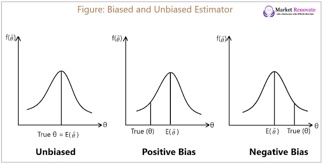
1. Unbiasedness (U): An estimator is unbiased if its expected value equals the population parameter’s true value. In other words, if we took multiple samples from the same population and calculated the estimator’s value for each, the average of those values would equal the true value of the population parameter. Unbiased estimators do not systematically overestimate or underestimate the population parameter. In small samples, unbiasedness is important because biased estimators can be more problematic due to the influence of outliers and random variation.

Suppose we want to estimate the average height of students in a school. We select a random sample of 20 students and compute the sample mean height, which is 170 cm. If the true average height of all students in the school is 170 cm, the sample mean is a fair estimate of the population mean.

Bias = Expected Value - True Value Bias = E(θ̂) - θ

θ̂ = Theta Hat

An estimator is said to be unbiased if,

E(θ̂) – θ = 0

∴ E(θ̂) = θ

But, if E(θ̂) > θ, it is a positive, upward bias.

If E(θ̂) < θ, it is a negative, downward bias.

2. Minimum or Least Variance (B): An estimator’s variance measures how much its estimates differ from sample to sample. A minimum or least variance estimator is preferred because it provides the most precise estimates. To put it another way, it reduces the amount of random error in the estimates. Estimators may have higher variance in small samples, making them less precise and reliable.

Continuing with the previous example, let us assume that the true population variance of student heights is 25 cm². There are numerous methods for estimating population variance, but one common estimator is the sample variance. If we use the sample variance to estimate the population variance, we should select a sample that minimizes the estimator’s variance.

For example, if a sample of 20 students has a sample variance of 30 cm², the estimator has more variance than a sample of 30 students with a sample variance of 20 cm². The sample of 30 students has a lower variance and thus is a better estimator in this case.

Let θ̂ is the best estimator of θ if,

var (θ̂) ≤ var ()

Where, is any other estimator of θ.

3. Minimum Mean Square Error (MSE): An estimator’s mean square error measures how far its estimates deviate from the true value of a population parameter on average. An estimator with the lowest mean square error is preferred because it provides the most accurate estimates. The mean square error is calculated by averaging the squared differences between the estimator’s value and the population parameter’s true value. To minimize the amount of error in the estimates, it is critical to use an estimator with a minimum mean square error in small samples.

Let us say we want to estimate the true proportion of voters who support a particular political candidate. We select a random sample of 100 voters and compute the sample proportion, which is 0.55. If the true proportion is 0.6, the sample proportion is not an unbiased estimator because it understates the true value systematically. However, we can calculate the minimum mean square error estimator using the bias-corrected estimator, which is the sample proportion plus a correction factor.

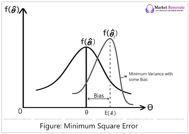
MSE (θ̂) = E(θ̂ - θ)²∴ MSE (θ̂) = var (θ̂) + [Bias (θ̂)]²

If Bias (θ̂) = 0, MSE = var (θ̂), but for minimum variance, we must accept some bias. In the figure below, f(θ̂₁) is unbiased, but it has no minimum variance, but f(θ̂₂) has minimum MSE but with some bias.

4. Efficiency (E): Efficiency (E) is a measure of how well an estimator uses the available data to estimate the population parameter. More efficient estimators are preferred because they provide more accurate estimates with less variability. Efficiency is especially important in small samples because less information is available to estimate the population parameter. An efficient estimator is one with the lowest variance among all unbiased estimators.

θ̂ is an efficient estimator if it satisfies the following two conditions:

a) E(θ̂) = θb) var (θ̂) ≤ var (), where  is any other unbiased estimator of θ.

Let us suppose we want to estimate the average salary of all employees in a large company. This parameter can be estimated using a simple random sample of employees. If we have two estimators, one with a larger variance and one with a smaller variance, the smaller variance estimator is more efficient.

5. Linearity (L): A linear estimator is one that is a linear combination of the sample data. Linearity is necessary to ensure that the estimator is simple to compute and interpret. A linear estimator is one that can be written as the sum of the sample data times a constant. This property makes it simple to understand how changes in the sample data affect the estimator.

Sample mean (θ̂)

= (∑x_i)/n

= 1/n[x₁ + x₂ + x₃ + .............. + x_n]

Sample mean (θ̂)

= (1/n)x₁ + (1/n)x₂ + (1/n)x₃ + .............. + (1/n)x_n

In this case, each observation is related in linear form of x's.

For example, we want to estimate the average temperature in a city over a given period of time. A linear estimator, which is a weighted sum of the daily temperatures during that time period, can be used. We could, for example, assign weights to each day based on its distance from the time period’s midpoint.

6. Best, Linear, Unbiased, and Efficient Estimator (BLUE): The BLUE estimator is best, linear, unbiased, and efficient estimator. In other words, the estimator provides the most accurate and precise estimates while remaining simple to compute and interpret. The BLUE estimator is preferred because it combines all desirable estimator properties. It is critical to use the BLUE estimator in small samples to ensure that the estimates are as accurate and precise as possible.

Let us say we want to estimate the true average weight of all cats in a certain breed using the Best, Linear, Unbiased, and Efficient Estimator (BLUE). The sample mean can be used as an estimator, but there are many other options, such as the median or mode. The sample mean, on the other hand, is the BLUE estimator because it is both unbiased and efficient.

7. Sufficiency: A statistic is sufficient if it contains all of the information needed to estimate the population parameter in the sample. In small samples, sufficiency is important because it ensures that the estimator uses all available information to estimate the population parameter. A sufficient statistic is one that contains all of the population parameter information contained in the sample.

This property enables the estimator to use only a subset of the sample data, which can be useful in situations where computing the estimator would be difficult or time-consuming otherwise.

Suppose we want to estimate the true average household income in a specific city. This parameter can be estimated using a simple random sample of households. However, we do not have to use all of the information in the sample. Instead, we can estimate the population parameter using a sufficient statistic, such as the sample mean or median, which contains all of the necessary information.

For example, the sample mean (x̄) is a sufficient estimator of the population mean (µ) since all the information in the sample is used in its calculations.

B. Large Sample Properties of Estimators

1. Asymptotic Unbiasedness: An estimator is said to be asymptotically unbiased when its expected value approaches the true population value as the sample size approaches infinity. This means that as sample sizes grow larger, the estimator becomes more accurate and unbiased. For example, the sample mean is an asymptotically unbiased estimator of the population mean because it approaches the true population means as the sample size increases.

An estimator θ̂ is said to be an asymptotically unbiased estimator of θ, if

Asymptotic bias of

2. Consistency: An estimator is consistent if it approaches the true population value in probability as the sample size approaches infinity. In other words, as the sample size increases, the probability of the estimator being far off from the true value decreases. The sample mean, for example, is a consistent estimator of the population mean because as sample size increases, the probability of the sample means deviating from the true population mean approaches zero.

For Consistency

concistency-property-of-large-sample-estimator

3. Asymptotic efficiency: Asymptotic efficiency is achieved when an estimator achieves the smallest possible variance among all consistent estimators. In other words, the estimator with the lowest variance is the most efficient for large sample sizes. For example, the maximum likelihood estimator is an asymptotically efficient estimator because it achieves the smallest possible variance among all consistent estimators as the sample size increases.

An estimator θ̂ is an asymptotic efficient estimator of the true population parameter θ, if θ̂ is consistent and if θ has a smaller asymptotic variance than any other consistent estimator.

Symbolically, θ̂ is efficient if,

Where, is any other consistent estimator of θ.

4. Asymptotic Normality: An estimator’s sampling distribution approaches a normal distribution as the sample size approaches infinity. This property is significant because it enables us to make inferences about the population parameter using inferential statistics.

The sample mean, for example, is asymptotically normally distributed due to the central limit theorem, which states that as sample size increases, the distribution of the sample means approaches a normal distribution.

5. Sufficiency: Sufficiency is another large sample property of estimators. A sufficient statistic contains all of the information needed about the population parameter. In other words, if we have sufficient statistics, we do not need to use all of the information in the sample to estimate the population parameter.

For example, because it contains all the necessary information about the mean, the sample mean is a sufficient statistic for estimating the population means. This property is significant because it allows us to reduce the data’s dimensionality and simplify the estimation process.

Suggested Articles:

Properties of Estimators - Small Sample and Large Sample